Numpy 1

Learning Objectives

• Load a Python library and use the things it contains.
• Read tabular data from a file into a program.
• Select individual values and subsections from data.
• Basic mathematical operations on arrays.
• Boolean questions on arrays.

We are going to hit the ground running and import some numerical data. In this case, we have a csv (comma separated variable) file containing historical price and volume data from the Nasdaq Stock Exchange (to be precise, the Nasdaq Composite index). This tutorial assumes the data is located in the followinf relative path: data/nasdaq.csv.

In order to load our data, we will use a function from library NumPy (hereafter numpy). In general you should use this library if you want to do analysis things numbers (Numpy is no good with textual data).

We can load numpy using:

import numpy as np

Importing a library is like getting a piece of lab equipment out of a storage locker and setting it up on the bench. Libraries provide additional functionality to the basic Python package, much like a new piece of equipment adds functionality to a lab space. Once you've loaded the library, we can ask the library to read our data file for us:

np.loadtxt('data/nasdaq.csv', delimiter=',', skiprows=1, usecols=(4,5))

array([ 5227.209961,  5213.220215,  5222.990234, ...,   100.760002,
         100.839996,   100.      ])

The expression np.loadtxt is a function call] that asks Python to run the function loadtxt that belongs to the numpy library.

This dotted notation is used everywhere in Python to refer to the parts of things as thing.component.

np.loadtxt has a number of parameters. Most importantly, the the name of the file we want to read, and the delimiter that separates values on a line. These both need to be character strings (or strings, so we put them in quotes.

By default, only a few rows and columns are shown (with ... to omit elements when displaying big arrays). To save space, Python displays numbers as 1. instead of 1.0 when there's nothing interesting after the decimal point.

Our call to numpy.loadtxt read our file, but didn't save the data in memory. To do that, we need to assign the array to a variable

Just as we can assign a single value to a integer,or list, or string (native data types) we can also assign an numpy array to a variable using the same syntax. Let's re-run numpy.loadtxt and save its result:

filepath = 'data/nasdaq.csv'
data = np.loadtxt(filepath, delimiter=',', skiprows=1, usecols=(4,5))

We also put the file path into a variable calledfilepath, which can help make the call to np.loadtxt a bit simpler.

Also, notice we supplied a function argument skiprows, and usecols. Depending on you file, these paramters might be useful, or critical, or both. But this is a bit of an aside, we'll cover this in more detail in the I/O section.

Accessing our data

Now that our data is in memory, we can start doing things with it. First, let's ask what type of thing data refers to:

print(type(data))

<class 'numpy.ndarray'>

The output tells us that data variable currently refers to an N-dimensional array (numpy.ndarray) created by the NumPy library. These data correspond to historical temperature records from Europe. The rows are the years and the columns are the seasons.

We can see what its shape is like this:

print(data.shape)

(11495, 2)

This tells us that data has 11495 rows, and 2 columns (it is 2-dimensional). When we created the variable data to store our past climate data, we didn't just create the array, we also created information about the array, called attributes. This extra information describes data in the same way an adjective describes a noun. data.shape is an attribute of data which described the dimensions of data. We use the same dotted notation for the attributes of variables that we use for the functions in libraries because they have the same part-and-whole relationship.

If we want to get a single number from the array, we must provide an index in square bracket, similar to how we have worked with lists:

print('first value in data:', data[0, 0])

('first value in data:', 5227.2099609999996)

print('some random value in data:', data[250, 0])

('some random value in data:', 4683.919922)

Hopefully, data[0,0] reminds you a bit of the indexing scheme we used for lists. The obvious difference, however, is that we have now provided two numbers. In a two dimesional array, two numbers are required to uniquely identify each element (and in N-dimensions it will be N numbers).

Again, like lists, we count from zero: therfore if we have an MxN numpy array, its indices go from 0 to M-1 on the first axis and 0 to N-1 on the second. Because if this convention, indexing takes a bit of getting used to.

An index like data[250, 0] selects a single element of an array, but we can select whole sections as well. For example, we can select the first ten data points like this:

print(data[0:10, :])

[[  5.22720996e+03   1.59252000e+09]
 [  5.21322022e+03   1.76177000e+09]
 [  5.22299023e+03   1.56102000e+09]
 [  5.23233008e+03   1.41664000e+09]
 [  5.21891992e+03   1.59106000e+09]
 [  5.21220020e+03   1.51189000e+09]
 [  5.21768994e+03   1.71478000e+09]
 [  5.26008008e+03   1.54705000e+09]
 [  5.24460010e+03   1.56021000e+09]
 [  5.23837988e+03   1.63274000e+09]]

The slice 0:10 means, "Start at index 0 and go up to, but not including, index 10." Again, the up-to-but-not-including takes a bit of getting used to, but the rule is that the difference between the upper and lower bounds is the number of values in the slice.

We don't have to start slices at 0:

print(data[5:10, 0:2])

[[  5.21220020e+03   1.51189000e+09]
 [  5.21768994e+03   1.71478000e+09]
 [  5.26008008e+03   1.54705000e+09]
 [  5.24460010e+03   1.56021000e+09]
 [  5.23837988e+03   1.63274000e+09]]

We also don't have to include the upper and lower bound on the slice. If we don't include the lower bound, Python uses 0 by default; if we don't include the upper, the slice runs to the end of the axis, and if we don't include either (i.e., if we just use ':' on its own), the slice includes everything:

small = data[:5, 0:]
print('small is:')
print(small)

[[  5.22720996e+03   1.59252000e+09]
 [  5.21322022e+03   1.76177000e+09]
 [  5.22299023e+03   1.56102000e+09]
 [  5.23233008e+03   1.41664000e+09]
 [  5.21891992e+03   1.59106000e+09]]

What's in our array?

At this point we should think a little bit about what our numpy array actually contains. Fistly, why all that scienctific notation? When our array contains both large and small values, numpy defaults to printing this way. In this case, there si sufficient variation in the magnitude of our values to have triggered this prinitng option,

If you'd like to learn about overidding this behavior, have a search for examples of setting np.set_printoptions on .

Okay, what about the first column?

print(data[0:5,0])

[ 5227.209961  5213.220215  5222.990234  5232.330078  5218.919922]

These values represent the daily closing price for the Nasdaq composite index (how do we know this? - let's get back to that later). One thing you may notice is that these values look like floats (floating point numbers). Unlike lists, Numpy arrays can only contain numbers. Even more restrictive, each instance of an array can only have ony type or number...e.g. float, int, complex. To find out which type of data out array contains, we can write

data.dtype

dtype('float64')

We cannot change the data type of a sub-array, only the entire array.

data[0,0] = int(1500)
print(data[0,0])

1500.0

As this code block shows, numpy will always coerce numbers into the correct (i.e current) data type. Strings and other non-numeric objects, however, will fail:

data[0,0] = "hello"

---------------------------------------------------------------------------
ValueError                                Traceback (most recent call last)
<ipython-input-12-a09d72434238> in <module>()
----> 1 data[0,0] = "hello"

Plotting our data

Let's have a quick look at our data by making perhaps the simplest plot in all of Pythondom:

%pylab inline
plt.plot(data[:,0])

plot here...

That was pretty easy huh! If you've been following the market however, you may notice that our data was plotted backwards. This is simply becuase our csv file listed data from newest to oldest, and numpy naturally reads from top to bottom. Do we need to fix this? Perhaps. Can we fix this? Absolutely:

First, let's use some list slicing trickery:

data2 = data[::-1, :]

plt.plot(data2[:,0])

Numpy slicing slicing extends Python’s basic concept of slicing to N dimensions. It returns is a slice object (constructed by start:stop:step notation inside of brackets).

Here, we used extended slicing that reads 'take all rows from the beginning the end (data[:::, :]), but in reverse order, hence the negative (data[::-1, :]). Note that the follwing, all make the same slice:

data[:, :]
data[::, :]
data[::1, :]

Importantly in this instance we didn't make a copy of the data. This is a bit confusing actually. We actually returned a view of the original data object (also called a shallow copy). What this means is that changes to the original array will be reflected in the view objects of that original array. This is true of all slices in numpy:

c = np.array([0, 1, 2, 3, 4])
d = c[:3]
c[2] = 9
print(c)
print(d)

[0 1 9 3 4]
[0 1 9

But, if you recall, this was not how lists worked:

c = [0, 1, 2, 3, 4]
d = c[:3]
c[2] = 9
print(c)
print(d)

[0, 1, 9, 3, 4]
[0, 1, 2]

If this is confusing you (and it should), one very simply way to force a deep copy to be made (rather than a view or a shallow copy), is to use the copy() method:

c = np.array([0, 1, 2, 3, 4])
d = c[::-1].copy()
c[2] = 9
print(c)
print(d)

[0 1 9 3 4]
[4 3 2 1 0]

A deeper explaination of views and copies can be found here: https://docs.scipy.org/doc/numpy-dev/user/quickstart.html

Maths with arrays

A great feature of Numpy arrays is the ease of doing mathematical operations on your data. Arrays know how to perform common mathematical operations on their values. The simplest operations with data are arithmetic: add, subtract, multiply, and divide. When you do such operations on arrays, the operation is done on each individual element of the array.

doubledata = data * 2.0

will create a new array doubledata whose elements have the value of two times the value of the corresponding elements in data:

print('original:')
print(data)
print('doubledata:')
print(doubledata[0:5,])

original:
[[  5.22720996e+03   1.59252000e+09]
 [  5.21322022e+03   1.76177000e+09]
 [  5.22299023e+03   1.56102000e+09]
 ..., 
 [  1.00760002e+02   0.00000000e+00]
 [  1.00839996e+02   0.00000000e+00]
 [  1.00000000e+02   0.00000000e+00]]
doubledata:
[[  1.04544199e+04   3.18504000e+09]
 [  1.04264404e+04   3.52354000e+09]
 [  1.04459805e+04   3.12204000e+09]
 [  1.04646602e+04   2.83328000e+09]
 [  1.04378398e+04   3.18212000e+09]]

If, instead of taking an array and doing arithmetic with a single value (as above) you did the arithmetic operation with another array of the same shape, the operation will be done on corresponding elements of the two arrays.

Thus:

tripledata = doubledata + data

will give you an array where tripledata[0,0] will equal doubledata[0,0] plus data[0,0], and so on for all other elements of the arrays.

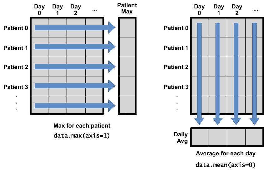
Often, we want to do more than add, subtract, multiply, and divide values of data. Arrays also know how to do more complex operations on their values. If we want to find the average value of all elements in an array, for example, we can just ask the array for its mean value

print(data.mean())

402558002.217

Numpy finds that the mean of our array, but remember this is all values of our array. Our data array contains two columns with differnt data (indeces), and a global mean is not meaningful. Instead we can do.

print(data.mean(axis=0))

[  1.33631733e+03   8.05114668e+08]

This gives us the average values 'down the columns'. Hence we end up with the average closing price of teh Nasdaq composit (column zero), and the avergage of daily volume (column one).

Numpy arrays have lots of useful methods:

print('maximum Nasdaq closing price:', np.max(data[:,0]))
print('minimum Nasdaq closing price:', np.min(data[:,0]))
print('mean Nasdaq closing price:', numpy.mean(data[:,0]))

('maximum Nasdaq closing price:', 5262.0200199999999)
('minimum Nasdaq closing price:', 54.869999)
('mean Nasdaq closing price:', 1336.3173298529796)

Questions of arrays

Okay, we've covered some basic numpy array accessing (indexing and slicing), as well as seen how easy basic mathematics. In line with the firts section of thise courses, a fundemental part of programming and data wrangling is being able to ask questions of our data. These questions generally evaluate to either true or false: the are known as boolean expressions, and as you may recall, Python has a special data type called Boolean, of which there are only two memebers (True and False)

x = np.array([1, 2, 3, 4, 5])

print('less than:') 
print( x < 3)
print('less than or equal:')
print( x <= 3)
print('equal:')
print(x == 3)
print('not equal:')
print(x != 3)

As you can see, these conditional or Boolean statements look exactly the same as when we used them on simpler variables, such as floats, in section 1.

less than:
[ True  True False False False]
less than or equal:
[ True  True  True False False]
equal:
[False False  True False False]
not equal:
[ True  True False  True  True]

print('are there any values greater than 4?') 
print(np.any(x > 4))

are there any values greater than 4?
True

print('are all values equal to six?')
print(np.all(x == 6))

are all values equal to six?
False

print('elements (indexes) where values are greater than 3:')
print(np.where(x > 3))

elements (indexes) where values are greater than 3
(array([3, 4]),)

print('original array indexed by elements where values are greater than 3')
print(x[np.where(x > 3)])

Let's return to teh Nasday data, and ask a question:

close = data[::-1,0].copy()
vol = data[::-1,1].copy()
print("Number days Nasdaq close above historical average average:")
print(np.sum(close > close.mean()))

Number days Nasdaq close above historical average average:
4788

Shell commands in the Jupyter notebook

!head -2 $filepath

Date,Open,High,Low,Close,Volume,Adj Close
2016-09-02,5249.660156,5263.390137,5231.02002,5249.899902,1474200000,5249.899902

Challenges

follow = close[:-1] < close[1:]