The Scipy library

Learning Objectives

• Introduce the diverse scipy tools
• Interpolation

SciPy is a collection of scientific functionality that is built on NumPy. The package began as a set of Python wrappers to well-known Fortran libraries for numerical computing, and has grown from there. The package is arranged as a set of submodules, each implementing some class of numerical algorithms. Here is an incomplete sample of some of the more important ones for data science:

• scipy.fftpack: Fast Fourier transforms
• scipy.integrate: Numerical integration
• scipy.interpolate: Numerical interpolation
• scipy.linalg: Linear algebra routines
• scipy.optimize: Numerical optimization of functions
• scipy.sparse: Sparse matrix storage and linear algebra
• scipy.stats: Statistical analysis routines

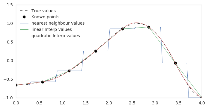
Interpolation of sparse data

Generally we use interpolation when we'd like to model data in between data points. The simplist type of interpolation is when our data is a function of 1 variable. This is often called Univariate interpolation in Scipy.

from scipy import interpolate
%pylab inline

Let's go ahead and create some data:

x = np.linspace(0, 4, 8)
y = np.cos(x**2/3+4)

xn = np.linspace(0, 4, 100)
y0 = np.cos(xn**2/3+4)

f1 = interpolate.interp1d(x, y, kind='linear')
f0 = interpolate.interp1d(x, y, kind='nearest')
f2 = interpolate.interp1d(x, y, kind='quadratic')


yn0 = f0(xn)
yn1 = f1(xn)
yn2 = f2(xn)

fig, ax = plt.subplots(figsize = (8,4))

ax.plot(xn, y0, '--k', label='True values', lw=0.7)
ax.plot(x, y, 'ok', label='Known points')
ax.plot(xn, yn0, label='nearest neighbour values', lw=0.7)
ax.plot(xn, yn1, label='linear Interp values', lw=0.7)
ax.plot(xn, yn2, label='quadratic Interp values', lw=0.7)

ax.legend(loc=2)
ax.grid()

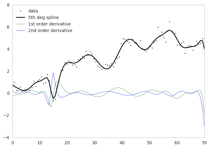
Gradients in noisy data

Often we would like to compute gradients in a data set. However, the gradient operator acts as a short pass filter, and enhaces high frequency noise. If your data contains a lot of high freqency noise, this will be amplified if we do not take care in how we calculate a gradient.

One solution is to smooth the original signal. Scipy’s UnivariateSpline class is a useful way to smooth 1-d data, such as time series, especially if you need an estimate of the derivative. It is an implementation of an interpolating spline.

Let's create some more data, this time with some random signal

np.random.seed(10)

# data
n = 100
x = np.linspace(0, 70, n)
y = 0.5 * np.cumsum(np.random.randn(n)) #Return a sample (or samples) from the "standard normal" distribution.

Import the 1-d Spline function from Scipy:

from scipy.interpolate import UnivariateSpline

k = 5 # 5th degree spline
s = 0.1*(n - np.sqrt(2*n)) # smoothing factor
spline_0 = UnivariateSpline(x, y, k=k, s=s)
spline_1 = UnivariateSpline(x, y, k=k, s=s).derivative(n=1)
spline_2 = UnivariateSpline(x, y, k=k, s=s).derivative(n=2)

y_sp0 = spline_0(x)
y_sp1 = spline_1(x)
y_sp2 = spline_2(x)

# plot data, spline fit, and derivatives
fig, ax = plt.subplots()

ax.plot(x, y, 'ko', ms=2, label='data')
ax.plot(x, y_sp0, 'k', label='5th deg spline')
ax.plot(x, y_sp1, 'g', label='1st order derivative', lw = 0.5)
ax.plot(x, y_sp2, 'b', label='2nd order derivative',  lw = 0.5)

ax.legend(loc='best')
ax.grid()